Guide
What Is Data Science? A Practical Forecasting Example
Follow a data science project from a business question to a tested one-week forecast, with eight fictional observations you can reproduce.
By the Space Office team · Published · Updated · 16 min read
Data science is the practice of combining statistics, computing, and subject knowledge to learn from data and make better-informed decisions. A project starts with a question and tests whether the available data supports a useful answer. This guide follows a print shop deciding how many pickup sleeves to prepare. In a scoped Space Office workflow, Lithium can implement an approved calculation, Carbon can check the results, and Hydrogen reviews the work before the shop owner decides whether to use it.

Key takeaways
- Write down the decision, prediction date, forecast horizon, and source of the eventual outcome.
- Choose a method that matches the question. A historical summary, a forecast, and an experiment require different evidence.
- Compare any forecast with a simple rule using information that was available at each prediction date.
- Report error in units the person making the decision can use, and inspect costly misses separately.
- Keep a human owner responsible for thresholds, overrides, and whether a pilot should proceed.
What does data science do?
A data science project connects three kinds of work. Subject knowledge establishes what the records mean and what the decision-maker can change. Statistics provides ways to describe patterns and estimate uncertainty. Computing makes it possible to transform records and repeat a calculation when fresh evidence arrives. A useful result could be a short estimate, an experiment design, or a tested forecast that someone can maintain. UC Berkeley School of Information on data science
Scroll horizontally to view all columns.
| Question | A method that fits | Evidence to request |
|---|---|---|
| What happened last month? | Describe the recorded outcomes by period and group. | Reconciled counts, metric definitions, and coverage. |
| What is likely to happen next week? | Forecast a named outcome at a fixed horizon. | Time-ordered evaluation against a simple baseline. |
| What would happen if we changed the policy? | Design an experiment or justify another credible comparison. | A clearly defined comparison, assignment process, and outcome window. |
| What action should we take? | Compare the cost and risk of feasible choices. | Decision limits, uncertainty, constraints, and a human owner. |
The print shop wants to prepare packaging for customer pickup orders. A retrospective report can show which weeks were busiest. A forecast can estimate next week’s pickup volume. A different question, such as whether a new pickup reminder increases collections, requires a comparison that supports a claim about the reminder. Even an accurate demand forecast would leave that question open. For the retrospective task, see the data analysis example.
Choose a result that can change an action. If the shop prepares every sleeve individually as the order arrives and has spare capacity all day, an aggregate weekly forecast may add little. If staff prep sleeves in batches on Friday and shortages interrupt Monday service, a one-week estimate can inform a real decision. Document which situation applies before asking for a model or dashboard.
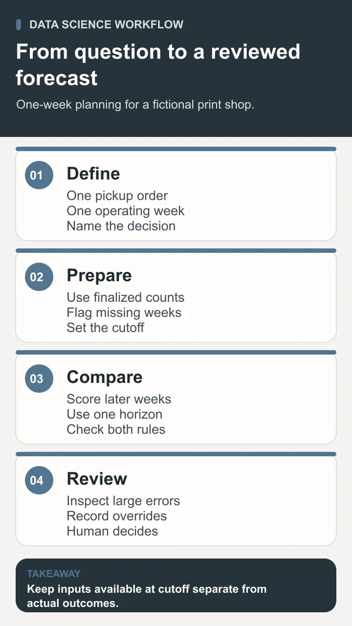
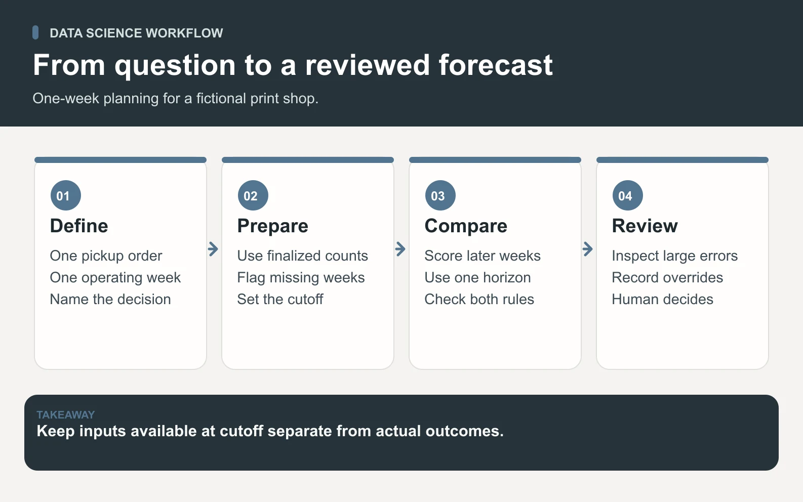
Define the decision and the data available at cutoff
The fictional shop decides on Friday how many reusable paper sleeves to prepare for the next week. The target is the total number of pickup orders that need a sleeve during that operating week. An order counted once uses one sleeve. Delivery orders are out of scope. The published example uses invented weekly counts and assumes that the previous week’s final count is available at each decision time. In a real shop, use the previous finalized period or test what could have been known at the actual cutoff.
Write down the time zone, the start and end of the operating week, the status used to count a pickup order, and which record proves completion. If a pending order can change fulfillment method, settle whether the final pickup or the original checkout selection controls the count. This choice determines which historical examples represent the outcome the shop actually wants to plan for.

- 1Start with one row per operating week, an order count, and a completion flag. Retain the source reference and extract time so a reviewer can reproduce the total.
- 2Distinguish an open week with zero orders from a closed week or an interrupted export. Keep closure and missing data visible as separate conditions.
- 3Check whether a physical limit hid demand. If staff turned away orders after supplies ran out, the recorded count may measure orders served rather than demand.
- 4Document which future facts would be known on Friday. A scheduled holiday can be known in advance. Next week’s actual pickups are available only after the week ends.
- 5Decide what to do when required inputs are late. The owner might use the existing preparation rule and record why the new forecast was skipped.
Compare two forecasts on eight fictional weeks
The invented counts for weeks 1 through 8 are 38, 42, 40, 44, 46, 42, 50, and 47. Compare a last-week forecast with a three-week trailing mean. The first rule carries forward the most recent observed count. The second takes the mean of the three most recent counts. The second rule gives a single unusual week less influence, at the cost of reacting more slowly when the level changes. A simple rule gives any later method a meaningful comparison. Forecasting: Principles and Practice on simple methods
Start the evaluation at week 5. For each target week, make a one-week-ahead prediction from the earlier observations and score it after the target is known. For week 5, the last-week rule uses 44. The trailing mean uses weeks 2, 3, and 4, so its prediction is (42 + 40 + 44) ÷ 3 = 42. Advance the cutoff one week and repeat. Each prediction uses the evidence available at its own cutoff. Forecasting: Principles and Practice on time-series cross-validation
Scroll horizontally to view all columns.
| Week | Actual orders | Last week | Last-week error | Three-week mean | Mean error |
|---|---|---|---|---|---|
| 5 | 46 | 44 | 2 | 42 | 4 |
| 6 | 42 | 46 | 4 | 43.33 | 1.33 |
| 7 | 50 | 42 | 8 | 44 | 6 |
| 8 | 47 | 50 | 3 | 46 | 1 |
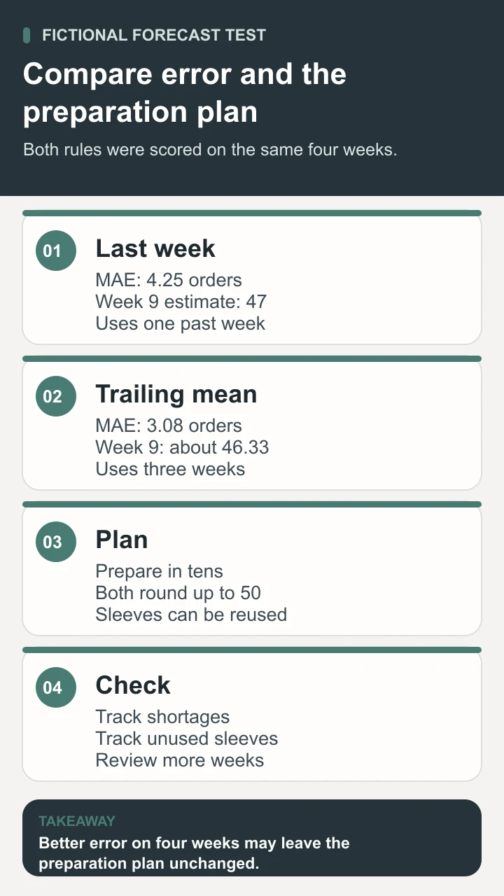
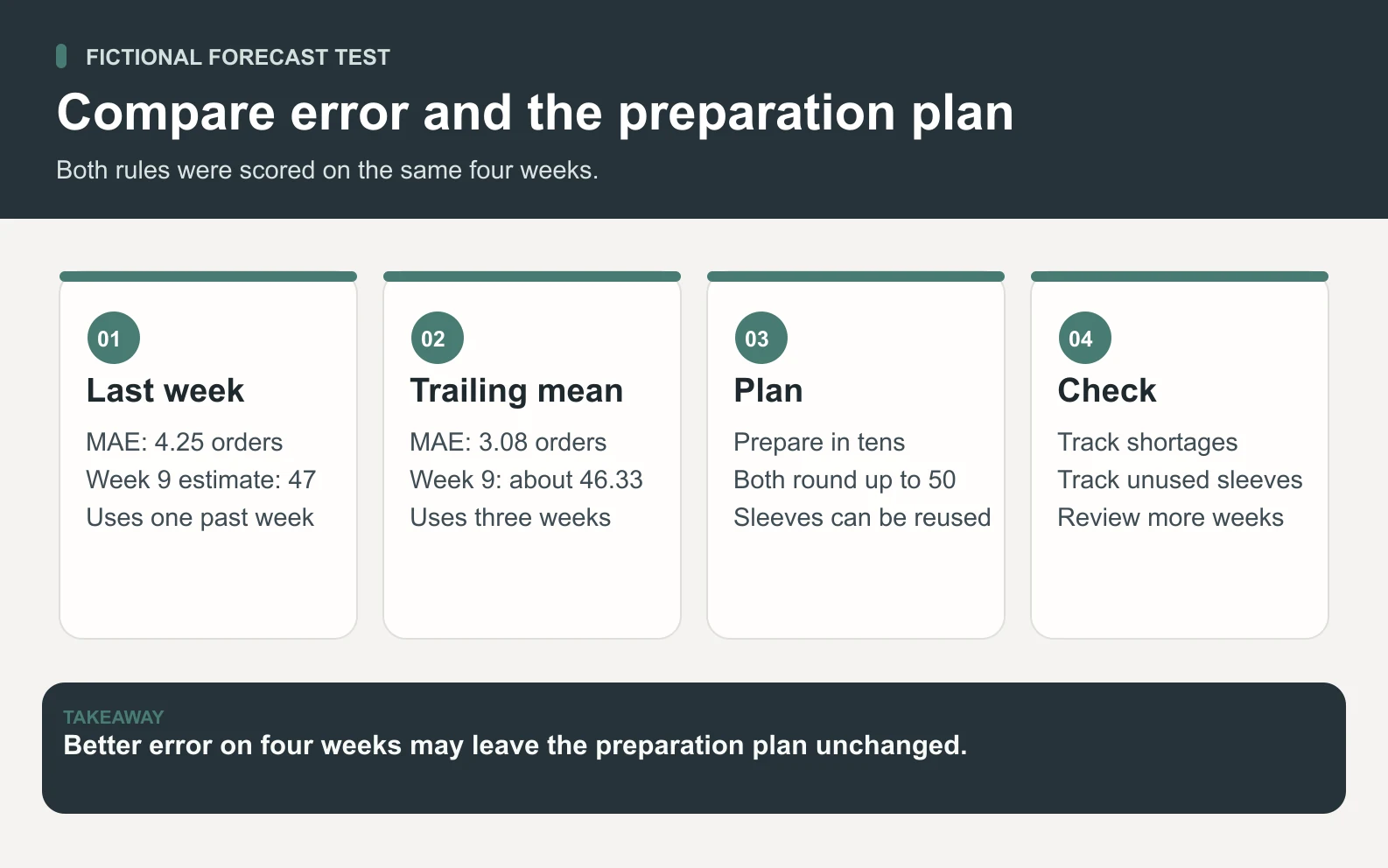
Calculate mean absolute error, or MAE, by averaging the four absolute differences between actual and predicted orders. The last-week rule has an MAE of (2 + 4 + 8 + 3) ÷ 4 = 4.25 orders. The trailing mean has an MAE of about 3.08 orders using unrounded values. The trailing mean performs better on these four fictional comparisons. That gives the reader a way to reproduce the calculation and a hypothesis to test on more evidence. Forecasting: Principles and Practice on forecast accuracy
For week 9, the last-week rule forecasts 47. The trailing mean uses 42, 50, and 47, which gives about 46.33. The shop prepares sleeves in bundles of ten. Its owner might prepare 50 for a trial week because excess plain sleeves can be reused. The difference between the two forecasts would lead to the same preparation decision under that policy. Check the effect on the actual action before investing in a more complicated method.
Download the forecast evaluation worksheet to reproduce the calculations and record your own decision cutoff. Keep forecast and actual in separate columns. The forecast column should remain fixed once the decision is made. Save the exact unrounded prediction for analysis and apply any bundle rounding in a separate planning column.
To reproduce the comparison in a spreadsheet, put week numbers in column A and actual counts in column B, with headers in row 1. Week 5 is row 6. In C6 enter =B5 for the last-week forecast. In D6 enter =AVERAGE(B3:B5) for the trailing mean. In E6 enter =ABS(B6-C6) and in F6 enter =ABS(B6-D6). Fill those four formulas through row 9. Average E6 through E9 and F6 through F9 separately. Check that every prediction formula references only rows above its own target row.
Run the two rules on the same completed weeks. If a week is missing, decide whether to skip any forecast that needs it or use an approved fallback and mark the row. The word trailing means the previous three weeks under the stated calendar. Taking the three most recent nonempty cells changes that definition and can quietly reach further back than intended. Retain a row for each week so missing values and closures are visible.
Check whether forecast errors matter to the decision
An average error treats overshooting and undershooting by the same amount equally. The shop cares differently about them. If shortages interrupt orders but leftover blank sleeves are reusable, understating demand can be more expensive. Review each signed error and record the operational effect before selecting a method. In week 7, the two rules undershoot by eight and six orders respectively. Either miss could matter if reserve stock is low.
Define the test horizon to match the action. A one-week estimate can help with total sleeve prep, but it does not tell the owner how many sleeves should be on the counter each day. A shop deciding Monday staffing would need daily counts and a test for that horizon. Likewise, training and checking a model on randomly mixed weeks could let information from the future influence a forecast intended to run in real time.
Watch for shifts that make past weeks less representative. A new pickup location, a change in product range, or a holiday can alter volume. Mark those periods and review performance separately where there are enough examples. When data are limited, scenario planning can communicate what would happen under several plausible volumes. Four example errors are too little evidence for a reliable prediction interval.
A useful review includes a policy for stale data, an owner for overrides, and a threshold for returning to the existing rule. For example, run a shadow comparison where staff record the forecast alongside their normal plan while keeping the old process in use. Record shortages, leftover sleeves, and unusual events after each week. If the forecast never changes the choice, stop and reconsider the decision it was meant to support.

Keep a dated record for each trial week with the estimate, the plan staff would otherwise use, the actual volume, the number prepared, and the owner’s reason for an override. Suppose both rules lead to 50 prepared sleeves but staff run short during a morning rush. A weekly error score may still look acceptable. Check when sleeves were needed and whether an extra small batch would solve the problem with less effort. The log gives the team evidence to change the decision or the prediction horizon.
Treat data preparation as part of the evaluation. If you revise which order statuses count after seeing a difficult week, document the rule change and repeat the comparison from the same starting point. A second set of later weeks can help test a choice you made while reviewing the first set. Keep a clear distinction between rows used to select the rule and evidence collected after selection.
Make the handoff reviewable with Space Office
Start with a narrow brief. Give Hydrogen the owner’s question, a sanitized weekly file, the rules for which orders count, and the decision cutoff. Ask for an implementation of the two agreed calculations and a review packet that shows the rows used, the forecasts, and the errors. Supply a small approved fixture the reviewer can calculate by hand. Customer names and payment details are unnecessary for this task.
In the Space Office workflow, Hydrogen can assign Lithium, the Full Stack Developer, to implement the approved data preparation and calculation in a scoped script or application branch. Carbon, the Senior QA Engineer and Test Strategist, can check empty weeks, time boundaries, duplicates in the source, and agreement with the hand-calculated fixture. Hydrogen reviews whether the artifacts match the brief and flags unresolved data issues.
A human analyst or operations owner chooses the method and approves any operational use. If the owner asks for a file-based exercise, the team can work from the supplied sample. Any access to a repository, export, or test environment needs the appropriate authorization and scope. Forecast design and uncertainty interpretation remain human responsibilities in this example. See the live specialist roster for role details.
Choose the smallest result you can use and check
A data science project earns its place when it helps a person make a specific decision and the evidence can be inspected later. For the print shop, that means a dated forecast, an existing rule to compare it with, a clear cutoff, and a record of actual shortages and leftovers. Start with a reversible preparation decision and keep the owner’s overrides visible. A more complex method has a case when the simple rule misses in ways that matter and the team can test the change honestly.
Sources and review notes
Reviewed against the linked primary sources on the checked dates. Search features and citations are selected by their respective platforms; no placement is guaranteed.
Frequently asked questions
What is data science?
Data science is the practice of using statistics, computing, and subject knowledge to learn from data and support decisions. A project may produce a historical analysis, an experiment, or a predictive model. Its value depends on whether the result answers the original question under clear data and testing assumptions.
How do data science and data analysis relate?
Data analysis is the work of inspecting and interpreting data for a question. It is part of many data science projects. A data science project can also involve engineering a repeatable data process, evaluating a predictive method, and checking whether the result improves a decision after adoption.
Can a spreadsheet be enough for a data science project?
A spreadsheet can handle the eight-week exercise and make every formula visible. Choose a tool that preserves the source, cutoff, formulas, and version history. As input size or refresh complexity increases, a scripted calculation can make the same rules easier to reproduce and test.
Why compare a model with a baseline?
A baseline represents a simple method the team could actually use. Testing the baseline and candidate on the same cases shows whether added complexity improves performance. In a forecast, preserve the same cutoff and horizon for both so the comparison reflects the decision being made.
When is a small forecast ready for operational use?
Check how it behaves across representative periods, whether the error is acceptable for the action, and what happens when inputs are missing. A human owner should define overrides, fallback, and how results will be monitored. A limited shadow comparison can supply evidence before an operational change.